Bengali.AI Handwritten Grapheme Classification - Midway Blog
Team: Zzz…
Members: Cheng Zeng, Zhi Wang, Peter Huang
Comparing different CNN architectures
We compared the performance using the basic CNN model, Densenet121 and Densenet169, Resnet and Efficientnet. Basic CNN model and Densenet can give reasonable training accuracy while for Resnet and Efficient, it is not easy to find a local minimum (training is not stable). We finally choose Densenet121 since its training converges steadily and it gives good accuracy. Note that although Densenet169 is denser and has more parameters, we found significant overfitting with this model.
Overview of processed dataset
Before we go into details of the CNN model used in this competition, we look at some basic info of the preprocessed dataset. Each image is now of 64\(\times\)64\(\times\)1 size, and the entire dataset has been split to training and validation datasets.
IMG_SIZE=64
N_CHANNELS=1
print(f'Training images: {X_train.shape}')
print(f'Training labels root: {Y_train_root.shape}')
print(f'Training labels vowel: {Y_train_vowel.shape}')
print(f'Training labels consonants: {Y_train_consonant.shape}')

Densenet121 model
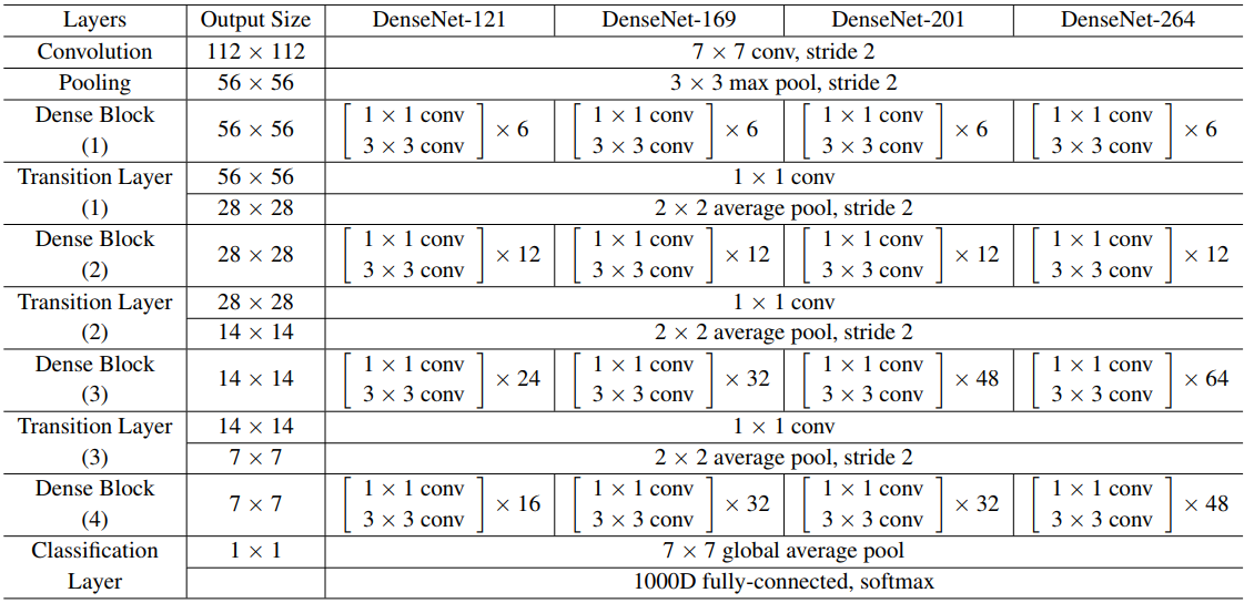
Densenet contains a feature layer (convolutional layer) capturing low-level features from images, several dense blocks, and transition layers between adjacent dense blocks.
Dense block
To reduce the computation, a 1\(\times\)1 convolutional layer (bottleneck layer) is added, which makes the second convolutional layer always has a fixed input depth. It is also easy to see the size (width and height) of the feature maps keeps the same through the dense layer, which makes it easy to stack any number of dense layers together to build a dense block. For example, densenet121 has four dense blocks, which have 6, 12, 24, 16 dense layers.
Transition layer
As a tradition, the size of the output of every layer in CNN decreases in order to abstract higher-level features. In densenet, the transition layers take this responsibility while the dense blocks keep the size and depth. Every transition layer contains a 1\(\times\)1 convolutional layer and a 2\(\times\)2 average pooling layer with a stride of 2 to reduce the size to the half. Be aware that transition layers also receive all the output from all the layers of its last dense block. So the 1\(\times\)1 convolutional layer reduces the depth to a fixed number, while the average pooling reduces the size.


Model construction
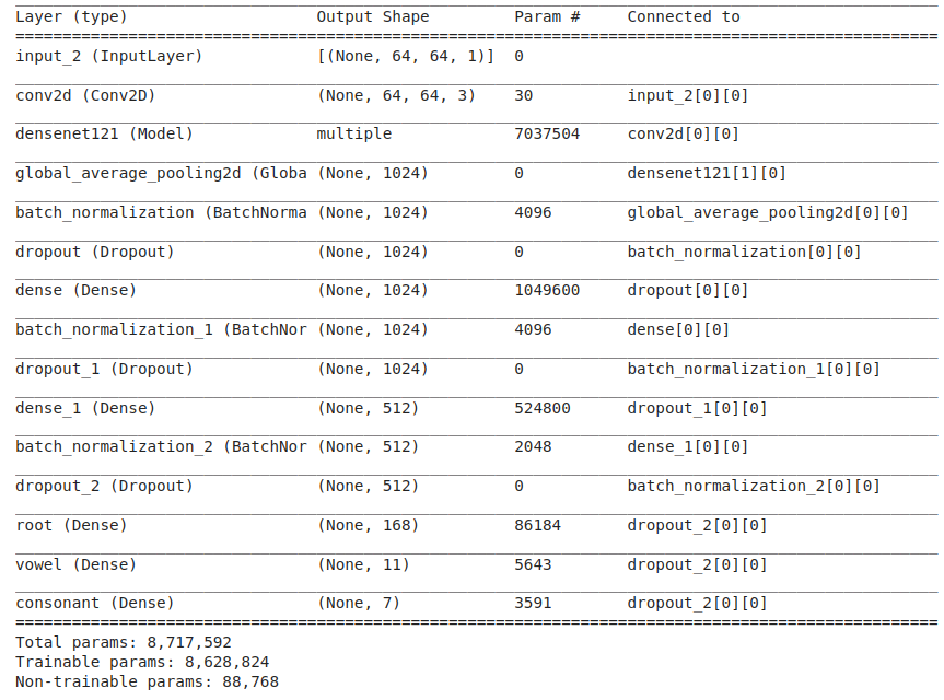
The model is constructed using the Densenet121 template implemented in TensorFlow. The model was built with deep learning API Keras. The code to construct the model is shown below.
def build_densenet(SIZE, rate=0.3):
    densenet = DenseNet121(weights='imagenet', include_top=False)

    input = Input(shape=(SIZE, SIZE, 1))
    x = Conv2D(3, (3, 3), padding='same')(input)

    x = densenet(x)

    x = GlobalAveragePooling2D()(x)
    x = BatchNormalization()(x)
    x = Dropout(rate)(x)
    x = Dense(1024, activation='relu')(x)
    x = BatchNormalization()(x)
    x = Dropout(rate)(x)
    x = Dense(512, activation='relu')(x)
    x = BatchNormalization()(x)
    x = Dropout(rate)(x)

    # multi output
    grapheme_root = Dense(168, activation = 'softmax', name='root')(x)
    vowel_diacritic = Dense(11, activation = 'softmax', name='vowel')(x)
    consonant_diacritic = Dense(7, activation = 'softmax', name='consonant')(x)

    # model
    model = Model(inputs=input, outputs=[grapheme_root, vowel_diacritic, consonant_diacritic])

    return model

model = build_densenet(SIZE=IMG_SIZE, rate=0.3)
Here we use a dropout rate of 0.3. Dropout is a regularization method, where a proportion of nodes in the layer are randomly ignored (setting their weights to zero) for each training sample. This drops randomly a proportion of the network and forces the network to learn features in a distributed way. This technique also improves generalization and reduces the overfitting.
Batch normalization is a technique for training very deep neural networks that standardizes the inputs to a layer for each mini-batch. This has the effect of stabilizing the learning process and dramatically reducing the number of training epochs required to train deep networks.
relu is short for rectified linear unit, which is an activation function defined as \(max(0,x)\). The rectifier activation function is used to introduce non-linearity into the neural networks.
A summary of the model can be seen if you run model.summary(); it should look like something below.

Optimizer and Learning schedule
We define the loss function to measure how poorly our model performs on images with known labels. It is the error rate between the observed labels and the predicted ones. We use a specific form for categorical classifications of multiple classes termed categorical_crossentropy.
Adam optimizer realizes the benefits of both AdaGrad and RMSProp. Instead of adapting the parameter learning rates based on the average first moment (the mean) as in RMSProp, Adam also makes use of the average of the second moments of the gradients (the uncentered variance). Specifically, the algorithm calculates an exponential moving average of the gradient and the squared gradient, and the parameters beta1 and beta2 control the decay rates of these moving averages.
The metric function accuracy is used is to evaluate the performance of our model. This metric function is similar to the loss function, except that the results from the metric evaluation are not used when training the model (only for evaluation).
Code for the setting the optimizer and fixed learning rate is shown below.
weights = {'root': 0.4, 'vowel': 0.3, 'consonant':0.3}
model.compile(optimizer=Adam(lr=0.00016), loss='categorical_crossentropy',
              loss_weights=weights, metrics=['accuracy'])
In order to make the optimizer converge faster and closest to the global minimum of the loss function, I used an annealing method of the learning rate (LR). The LR is the step by which the optimizer walks through the ‘loss landscape’. The higher LR, the bigger are the steps and the quicker is the convergence. However, the sampling is very poor with a high LR and the optimizer could probably fall into a local minimum. It’s better to have a decreasing learning rate during the training to reach efficiently the global minimum of the loss function.
# Learning rate will be half after 3 epochs if accuracy is not increased
lr_scheduler = []
targets = ['root', 'vowel', 'consonant']
for target in targets:
 lr_scheduler.append(ReduceLROnPlateau(monitor=f'{target}_accuracy',
                     patience=3,verbose=1,factor=0.5,
                     min_lr=0.00001))
# Callback : Save best model
cp = ModelCheckpoint('saved_models/densenet121_128x128_1-rr.h5',
monitor = 'val_root_accuracy',save_best_only = True,
save_weights_only = False,mode = 'auto',verbose = 0)
ModelCheckPoint is used to save the whole model or just the weights if our model improves by the criteria of improvement defined.
Data augmentation
In order to avoid the overfitting problem, we need to expand artificially our handwritten digit dataset. We can make your existing dataset even larger. The idea is to alter the training data with small transformations to reproduce the variations occurring when someone is writing a digit.
By applying just a couple of these transformations to our training data, we can easily double or triple the number of training examples and create a very robust model.
For the data augmentation strategies, I chose to:
- Randomly rotate some training images by 8 degrees
- Randomly Zoom by 15% some training images
- Randomly shift images horizontally by 15% of the width
- Randomly shift images vertically by 15% of the height
The improvement is critical:
- Without data augmentation, I obtained an accuracy of 81.85%, 95.02%, and 94.95% for respective grapheme roots, vowel diacritics and consonant diacritics.
- With data augmentation, I achieved an accuracy of 90.07%, 96.71%, and 97.11%.
Code for image augmentation is shown below.
# Data augmentation for creating more training data
datagen = MultiOutputDataGenerator(
    featurewise_center=False,  # set input mean to 0 over the dataset
    samplewise_center=False,  # set each sample mean to 0
    featurewise_std_normalization=False,  # divide inputs by std of the dataset
    samplewise_std_normalization=False,  # divide each input by its std
    zca_whitening=False,  # apply ZCA whitening
    rotation_range=8,  # randomly rotate images in the range (degrees, 0 to 180)
    zoom_range = 0.15, # Randomly zoom image
    width_shift_range=0.15,  # randomly shift images horizontally (fraction of total width)
    height_shift_range=0.15,  # randomly shift images vertically (fraction of total height)
    horizontal_flip=False,  # randomly flip images
    vertical_flip=False)  # randomly flip images
In the final blog, we will talk about the evaluation steps and methods to improve the model. Check the leaderboard results as well.