Jigsaw Multilingual Toxic Comment Classification - Start Blog
This is the first of three blogs documenting my entry into the toxic comment classification kaggle competition. It is a natural language processing (NLP) task. I chose this topic as the final project because NLP is a very hot topic nowadays and I am new to this area. I hope to take advantages of this opportunity to learn more about deep learning targeted towards the state-of-art application in NLP.
In the first blog, I walk you through an overview of the competition, the exploratory data analysis, and the basics of language models for this project.
Introduction
Background & Motivation
Thanks to the rapid development of deep learning techniques and computational hardwares, NLP has been gaining its momentum in the past two decades. As believed by machine learning experts, NLP is experiencing a boom in the short-term future, same as computer vision once did. The popularity of it brought a great amount of investment. Recently Kaggle released two NLP competitions (tweet sentiment extraction and comment toxicity analysis). Of focus here is the second one because it is based off two previous Kaggle competitions regarding the same topic (2018 toxicity and 2019 toxicity). For the very first competion, contestants are challenged to buld multi-headed models to recognize toxicity and several subtypes of toxicity. Toxicity is defined as anything rude, disrespectful or other wise likely to make someone leave a discussion. The 2019 Challenges asks Kagglers to work across a diverse range of conversations. The main purpose of this final project is to understand the basics of deep learning techniques applied to NLP. So it would be more doable to work on a project in such a limited time for which there exist many established references/documents.
Description of The Competition
Taking advantage of Kaggle’s TPU support, this competition aims to build multilingual models with English-only training data. The model will be tested on Wikipedia talk page comments in several different languages. It is supported by The Conversation AI team, which is funded by Jiasaw and Google.
Evaluation Metrics and Submission Requirements
Basically it is a classification problem. The model performance is evaluated by the area under the ROC curve between the predictions and the observations.
The submission file consists of two columns. The first column indicates the comment id and the second one is the probability for the toxicity variable. Following is a sample submission file.
| id | toxic |
|---|---|
| 0 | 0.3 |
| 1 | 0.7 |
| 2 | 0.9 |
In addition to the well defined metrics evaluated on the given testing set. We might also want to further apply the language model to additional applications. For example,
-
As mentioned before, there is another NLP competition on Kaggle, which challenges contestants to analyze the tweet sentiment. Basically there are three types of sentiment, including neural, negative and positive.
-
Another possible application is to scrape comments from some social media, say “reddit”, and predict whether the comment will receive upvote, downvote or be removed.
Data Exploration
Dataset
Following is the list of the datasets we have for this project. The primary data is the comment_text column which contains the text of comment to be classified as toxic or non-toxic (0…1 in the toxic column). The trainingset’s comments are mostly written in English whereas the validation and testing sets’ comments are composed of multiple non-English languages. A detailed explanation of the dataset can be found on the competition web page

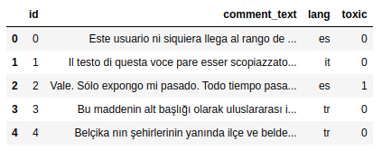
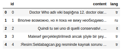
Below shows the five top rows of the training set, validation set and testing set. There are mainly four columns for all datasets, in which id is the identifier, commen_text is the text of comment, lang is the language of the comment, and toxic is whether or not the comment is toxic. In the training set, we can see 5 additional columns which represent the subtypes of toxic comment. Moreover, we do not have the toxic column in the testing set.
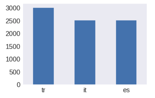
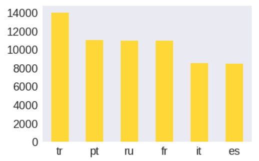
As mentioned before, most comments in the training set are in English while most comments in validation and testing set are in Non-English, including Spanish, French, Turkish and Portuguese etc. The number for all types of languages in validation and test set are summarized at below.
Preprocessing
We can do a few data preprocessing steps before feeding the data into a language model.
-
Clean up the comment texts by dropping redundant information, such as usernames, emails, hyperlinks and line breakers.
-
Remove unnecessary columns in the trainingset such as the subtypes of toxicity because the target for submission is only the
toxic. -
Tokenize the words, which can be also considered as a step for building up a model.
Exploratory data analysis (EDA)
Note that the analysis for “wordcloud” is inspired by this kernel EDA and Modeling Kernel.
Comment Wordcloud
Firstly we take a look at the comments in the training set.
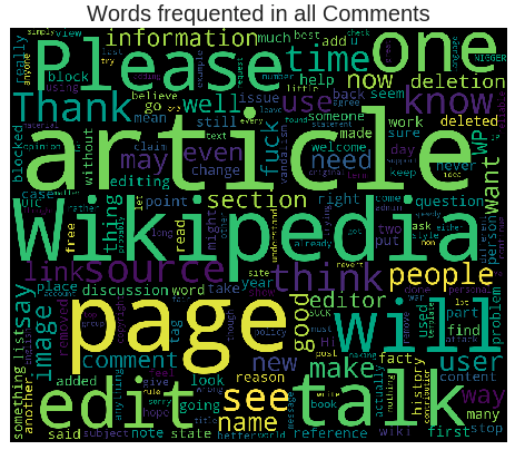
The most common words include “Wikipedia”, “article”, “will” and “see”.
Another plot in the following shows the wordcloud for common words in the toxic comments.
WARNING
The following figure contains text that may be considered profane, vulgar, or offensive.
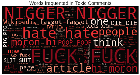
As expected, there exist more insulting or hateful words, such as “die” and “pig”.
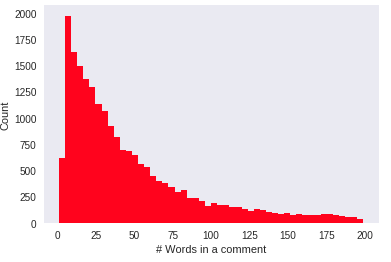
Histograms of number of words and sentences in all comments
The figure below shows the distribution for number of words in all comments. One can see that the distribution is right-skewed, and it is peaked at 13 words per comment.
Histogram of number of sentences in all comments
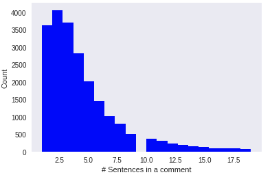
The distribution for number of sentences is also right skewed.
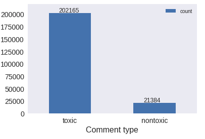
Balance of training set
This bar plot indicates that the balance of the dataset is about 90%. The dataset is hence highly unbalanced.
Basics of Language Models
What is a Language Model?
A language model is basically a machine learning model that looks at part of a sentence and is able to predict the next one, such as next word recommendation for cellphone keyboard typing.
Statistically, a language model is a probability distribution over sequence of words. Most language models rely on the basic assumption that the probability of a word only depends on the previous n words, which is known as the n-gram model. Language models are useful in many scenarios such speech recognition, parsing and information retrieval. Please refer to the Wiki page for more information.
Word Embeddings
Word embedding is a type of word representation that allows words with similar meaning to have a similar representation. It is a groundbreaking progress for developing high-performance deep learning models for NLP. The intuitive approach to word representation is the one-hot encoding. To represent each word, we create a zero vector with length equal to the vocabulary. Then one is placed in the index that corresponds to the word. In that sense, we will create a sparse vector. An alternative approach is to encode each word with a unique number so that the resulting vector is short and dense. However, the way how each word is encoded is arbitrary, and we do not know the relationship between the words. Here comes the technique of word embeddings. In this scenario, we do not have to specify the encoding by hand. Instead of manually defining the embedding vector, the values of the vector are trained in the same way a model learns weights of a dense layer. A high-dimensional embedding can capture fine relationships between words.
Attention
The key idea of Attention is to focus on the most relevant parts of the input sequence as needed. It provides a direct path to the inputs. So it also alleviates the vanishing gradient issue. This significantly improves the model performance when confronting with long sentence analysis.
For a typical language model, it is composed of an encoder and a decoder. The encoder processes each item in the input sequence, and then compile the transformed information into a vector. After processing the entire input sequence, the encoder send the context to the decoder for the next step. Both the encoder and decoder are intrinsically recurrent nueral networks (RNN) which processes the input vector and previous hidden state, and produces the next-step hidden state and output at that time step.
At a high level of abstraction, an attention model differs in two main ways. Firstly, instead of passing only the last hidden state at the encoder side, the attention model holds all the hidden states and passes all hidden state to the decoder. Secondly, in the decoder side it does one more step before calculating its output. The basic idea is that each hidden state produced at the encoder side is associated with a certain word in the input sequence, thus we can assign a score to each hidden state and use that to amplify the word with high score and drown out words with low scores. A illustrative and comprehensive tutorial of an attention model can be found in the blog visualizing a neural machine translation model.
Annotated Citations
-
Tarun Paparaju. (2020, March). Jigsaw Multilingual Toxicity : EDA + Models. Retrieved from https://www.kaggle.com/tarunpaparaju/jigsaw-multilingual-toxicity-eda-models. The function for plotting the WordCloud is adapted from this kernel.
-
Jay Alammer. (2018, May 9). Visualizing A Neural Machine Translation Model. Retrieved from https://jalammar.github.io/visualizing-neural-machine-translation-mechanics-of-seq2seq-models-with-attention/. Some explanation for attention comes from this blog.
-
Barry Clark. (2016, March). Build a Jekyll blog in minutes, without touching the command line. Retrieved from https://github.com/barryclark/jekyll-now.This site offers the github page template using
Jekyll. -
Jason Brownlee. (2017, October 11). What Are Word Embeddings for Text? Retrieved from https://machinelearningmastery.com/what-are-word-embeddings/. This site provides some examples to explain the idea of word embedding.
-
Mohammed Terry-Jack. (2019, April 21). NLP: Everything about Embeddings. Retrieved from https://medium.com/@b.terryjack/nlp-everything-about-word-embeddings-9ea21f51ccfe. More explanation about the word embedding can be found in this Medium blog.
-
Anusha Lihala. (2019, March 29). Attention and its Different Forms. Retrieved from https://towardsdatascience.com/attention-and-its-different-forms-7fc3674d14dc. The original attention and its variants are detailed and compared in this Medium blog.
-
Sean Robertson. (2017). NLP FROM SCRATCH: TRANSLATION WITH A SEQUENCE TO SEQUENCE NETWORK AND ATTENTION. Retrieved from https://pytorch.org/tutorials/intermediate/seq2seq_translation_tutorial.html. Code implementation in the framework of
PyTorchis discussed in this web page.