Jigsaw Multilingual Toxic Comment Classification - Midway Blog
This blog is the second of the three blogs documenting my entry into toxic comment classification kaggle competition. In the first blog, we introduced the dataset, the EDA analysis and some fundamental knowledge about a language model. To move forward, the primary purpose of the next step is to develop the baseline model from scratch. The link is provided in the notebook for the model or running it on colab. The essential components of a language model are summarized, including the tokenizer, the model architecture, and the evaluation metrics. In addition, we will cover some state-of-the-art multilingual models, such as BERT, XLM and XLM-RoBERT.
The Baseline Model
Our goal is to take a comment text as input, and produces either 1(the comment is toxic) or 0 (the comment is non-toxic). It is basically a binary classification problem. The simplest model we can think of is the logistic regression model, for which we need to figure out how to digitalize comments so that we can use logistic regression to predict the probabilities of a comment being toxic. Next we will do a quick overview of the dataset, introduce the concepts of tokenizer, and go over the architecture of a baseline model.
Dataset: Jigsaw Multilingual Comments
The dataset we will use, as mentioned in the first blog, is from the Kaggle competition Jigsaw Multilingual Toxic Analysis, which contains the comment texts and its toxicity labels, indicating whether the comment text is disrespectful, rude or insulting.
| Comment | Toxic |
|---|---|
| This is so cool. It's like, 'would you want your mother to read this??' Really great idea, well done! | 0 |
| Thank you!! This would make my life a lot less anxiety-inducing. Keep it up, and don't let anyone get in your way! | 0 |
| This is such an urgent design problem; kudos to you for taking it on. Very impressive! | 0 |
| haha you guys are a bunch of losers. | 1 |
| Is this something I'll be able to install on my site? When will you be releasing it? | 0 |
We can load the dataset with pandas. Then we split the dataset to train and test sets in a stratified fashion as the dataset is highly unbalanced.
The splitting ratio is 8:2.
import numpy as np
import pandas as pd
from sklearn.model_selection import train_test_split
train = pd.read_csv("./jigsaw-toxic-comment-train.csv")
X, y = train.comment_text, train.toxic
X_train, X_test, y_train, y_test = train_test_split(X, y, test_size = 0.2, random_state = 42, stratify=y)
y_train, y_test = y_train.astype(int), y_test.astype(int)
Tokenizer
A tokenizer works as a pipeline. It processes some raw text as input and output encoding. It is usually structured into three steps. Here we illustrate the idea of tokenization by the example provided in the blog “A Visual Guide to Using BERT for the First Time”. For instance, if we would like to classify the sentence ““a visually stunning rumination on love”, the tokenizer will firstly split the sentences into words with some separator, say whitespace. In the next step, special tokens will be added for sentence classifications for some tokenizers.
The final step is to replace each token with its numeric id from the embedding table, which is a natural component of a pre-trained model. Then the sentence is ready to be sent for a language model to be processed.
For the purpose of demonstration, in the baseline model, we will use a classic tokenization method TF-IDF, which is short for “term frequency-inverse document frequency”. Basically it counts the number of occurrence of a word in the documents, and then it is offset by the number of documents that contain the word. This tokenization approach is available in the package sklearn.
### Define the vectorizer
from sklearn.feature_extraction.text import TfidfVectorizer
tfidf_vectorizer = TfidfVectorizer(max_features=2000, min_df=2, max_df=0.95)
### Suppose X_train is a corpus of texts
## Fit the vectorizer
X_train_fitted = tfidf_vectorizer.fit_transform(X_train)
X_test_fitted = tfidf_vectorizer.transform(X_test)
In addition, HUGGING FACE provides a open-source package, named tokenizer, where you can find many fast state-of-the-art tokenizers for research and production. For example, to implement a pre-trained DistilBERT tokenizer and model/transformer, you just need two-line codes as follows
import transformers as ppb
# For DistilBERT:
tokenizer_class, pretrained_weights = (ppb.DistilBertTokenizer, 'distilbert-base-uncased')
# load pretrained tokenizer
tokenizer = tokenizer_class.from_pretrained(pretrained_weights)
After tokenization, we can build a model and train it with the tokenized comments.
The Model
We define the simplest binary classification model with logistic regression.
from sklearn.linear_model import LogisticRegression
# C is a term to control the l2 regularization strength
model_lr = LogisticRegression(C=6.0)
If you want to optimize the hyperparameter C, you can do a simple grid search.
from sklearn.model_selection import GridSearchCV
parameters = {'C': np.linspace(0.0001, 100, 20)}
grid_search = GridSearchCV(LogisticRegression(), parameters)
grid_search.fit(X_train_fitted, y_train)

print('best parameters: ', grid_search.best_params_)
print('best scrores: ', grid_search.best_score_)
We train and evaluate the model by the prediction accuracy. Note the official metric for this competition is ROC-AUC, which is more reasonable for a highly unbalanced dataset.
## training
model_lr.fit(X_train_fitted, y_train)
## prediction on testing set
model_lr.score(X_test_fitted, y_test)
Note that Tfi-df tokenization is not capable of dealing with multiple languages. Instead we should refer to other tokenizers, for example a BERT tokenizer. The example using bert-base-uncase model and tokenizer can be found in this colab notebook.
Cross-lingual Models
BERT
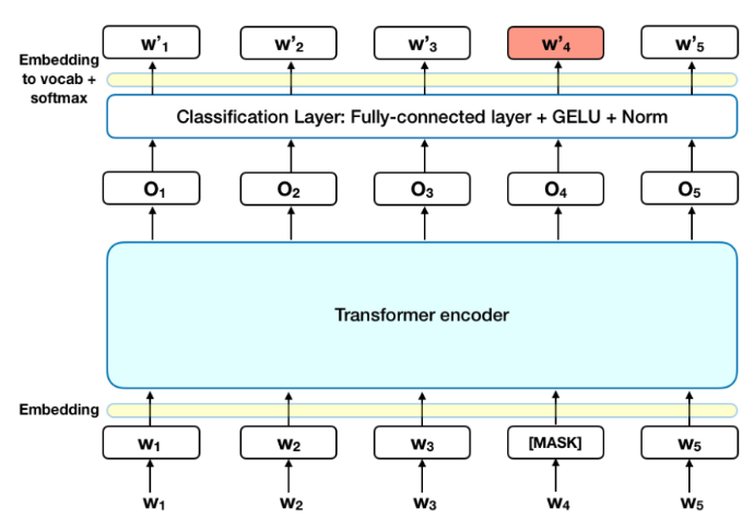
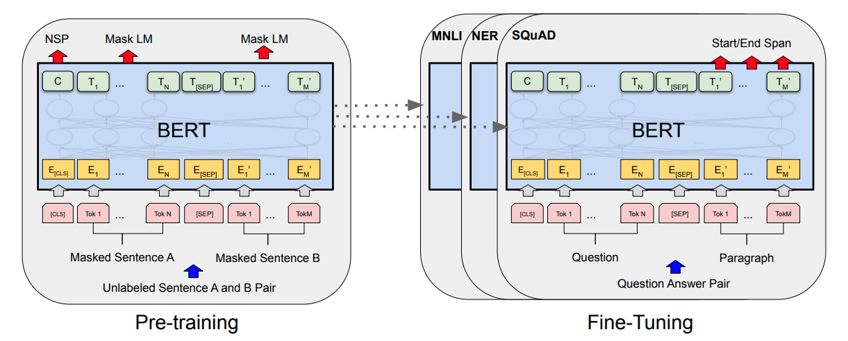
BERT, which stands for Bidirectional Encoder Representations from Transformers, have achieved great success in Natural Language Processing. In contrast with previous language models looking at a text sequence from left to right, the innovation of BERT lies in that it is designed to train bidirectional representation by jointly conditioning on both the left and right context. The following figure shows a high-level description of the BERT architecture. It is essentially a stack of Transformer encoders. The input is a ‘sentence’ which is tokenized and word-embedded with a 30,000 token vocabulary. The output is a sequence of vectors, for which each vector represents an input token with the same index.

It is natural that a language model typically looks at part of the sentence and predict the next words. However, it is challenging to define prediction tasks when we look at the sentence bidirectionally.
The authors of the original paper uses two pretraining techniques to overcome this issue. They are both unsupervised approaches, namely masked language modeling (MLM) and next sentence prediction (NSP).
Masked Language Modeling
15% of the words in a sentence are masked with a [MASK] token. Then the model tries to predict the original tokens in the masked positions. In practice, BERT implemented a more statistically mask scheme. For more details, please refer to the Appendix C
Next Sentence Prediction (NSP)
In BERT, the model can take two sentences as input, and learned to predict if the second sentence of the pair sentences is the subsequent or antecedent. During pretraining, for 50% of the pair sentences, the second sentence is the actual next sentence, whereas for the rest 50%, the second sentence is randomly chosen, which is supposed to be disconnected from the first sentence.
The pretraining is conducted on documents from BooksCorpus and English Wikipedia. In this scenario, a document-level corpus is used to extract long sequences.
Fine tuning
The fine tuning process refers to using the pretrained BERT to do a downstream task. The process is straightforward and task specific. The architecture is the same except the output layers. Although during fine-tuning, all parameters are fine-tuned, it turns out that most parameters will stay the same.

In order to get a in-depth understanding of this technique, we highly recommend reading the paper, or the open source code by Google research.
XLM
Though BERT is trained on over 100 languages, it was not optimized for multilingual models since most of its vocabulary does not commute between languages, and as a result, the knowledge shared is limited. To overcome this issue, instead of using word or characters as input, XLM uses Byte-Pair Encoding (BPE) that splits the input into the most common sub-words across all languages (see BPE wiki page for more details about this data compression technique).
Intrinsically XLM is a updated BERT techniques. It updates BERT architecture in two ways.
-
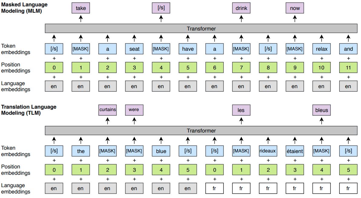
Each training sample consists of the same text in two languages. To predict a masked word in one language, the model can either attend to surrounding words in the same language or the other language. In this way, alignment between contexts of the two languages can be facilitated.
-
The model also uses language IDs and the order of the tokens in the format of positional embeddings to better understand the relationship of related tokens in various languages.
This new approach is named as Translation Language Modeling (TLM). The model pretraining is carried out as the following schematic representation.

The model is trained by using MLM, TLM or a combination of both.
XLM-RoBERTa
Similar to XLM, XLM-RoBERTa is also a transformer-based architecture, both relied on MLM and are capable of processing texts across 100 languages. However, the biggest update is that the new architecture is trained on way more data than the original one, i.e. 2.5 TB storage. And the ‘RoBERTa’ comes from that the training is the same as the monolingual RoBERTa model, for which the sole objective is the MLM, without NSP and TLM. COnsidering the diffuculties of using various tokenization tools for different languages, Sentence Piece model is trained at the first step and then it is applied to all languages. The XLM-RoBERTa model has demonstrated to be superior than the state-of-the-art multilingual models such as GermEval18.
Note that all the pretrained models mentioned above can be easily called by using Huggingface packages.
Annotated Citations
-
T. Kudo and J. Richardson. SentencePiece: A simple and language independent subword tokenizer and detokenizer for Neural Text Processing. 2018. This is a paper discussing various tokenization techniques.
-
Alexis Conneau and Kartikay Khandelwal et.al. Unsupervised Cross-lingual Representation Learning at Scale. 2020.The XLM-RoBERTa model originates from this paper.
-
Guillaume Lample and Alexis Conneau. Cross-lingual Language Model Pretraining. 2019. This paper is the first work using the XLM architecture for language modeling.
-
Jacob Devlin, Ming-Wei Chang, Kenton Lee and Kristina Toutanova. BERT: Pre-training of Deep Bidirectional Transformers for Language Understanding. 2019. This is the original paper for BERT architecture.
-
Jay Alammer. (2019, November 26). A Visual Guide to Using BERT for the First Time. Retrieved from BERT notebook. The vivid figures for illustration of key components in a language model are taken from this awesome blog.