Jigsaw Multilingual Toxic Comment Classification - Final Blog

This blog is the last of the three blogs documenting my entry into the toxic comment classification kaggle competition. In the first blog, we introduced the dataset, the EDA analysis and some fundamental knowledge about a language model. In the second blog, the simplest logistic regression model is taken as an example to illustrate the essential components of a language model. A multilingual classification model using BERT architecture is also developed. In addition, we went over state-of-the-art multilingual models, including BERT, XLM and XLM-RoBERTa. The novel techniques in each type of architecture are elaborated and compared.

This blog summarizes relevant techniques employed to improving the model performance, which is evaluated by the public leaderboard score on Kaggle. I will start with the basic BERT multilingual model, after which I will illustrate how we can improve the model by tackling the three main challenges for this competition.

Honestly this is my first NLP project. I chose a project on Kaggle because the Kaggle community is an awesome place to share and learn machine learning knowledge. I would like to thank all those great participants on Kaggle, who make this learning process so rewarding and enjoyable.

The Basic BERT Model

The Objective

Our goal is to take a comment text as input, and produce either 1(the comment is toxic) or 0 (the comment is non-toxic). It is basically a binary classification problem. There are three significant challenges regarding this competition that one needs to take care of.

• Data Size Issue: the training dataset consists of more than 200,000 data, which thus requires a huge amount of time to clean and pre-process the data. In addition, training on regular GPUs might not be able to give us a decent model in a limited time. For example ,the commit time should be less than three hours on Kaggle, which is almost impossible for a typical multilingual model of 100 million parameters to converge on such a large size dataset.

• Imbalance Issue: the training and validation set is highly unbalanced with a toxic/nontoxic ratio around 1:9. Therefore, this competition uses the ROC-AUC value as the evaluation metric. In other words, if we train the model based on the unbalanced dataset, the model should predict better on nontoxic comments than toxic ones.

• Multilingual Issue: the training set is written in English. The validation is given in three languages, Turkish, Spanish, and Italian. Besides the multilingual validation set, the testing set is written in three more types of languages, i.e. Russian, French and Portuguese.

We will discuss how we can circumvent or mitigate those three issues in the model refinement part.

Tokenizer, Transformer and Classifier

Simply for demonstration of a multilingual model, we will use the BERT tokenizer and transformer as implemented in the HuggingFace package. In the following we use the example illustrated in Jay’s awesome blog to show how we encode a comment text, pass it through the model and finally do the classification.

Tokenizer

The first step is to split the words into tokens. Then special tokens are added for the purpose of classification. For example, [CLS] is added as the first position of a comment/review, and [SEP] is added at the end of each sentence. Note that a comment/review may consist of many sentences, therefore we could have many [SEP]s in one comment, but only one [CLS].

Lastly, the tokens are embedded into its id using the embedding model-specific table component. As we mentioned in the second blog, BERT uses word-piece tokenization while XLM uses Byte-Pair Encoding to grasp the most common sub-words across all languages.

Now the input comment is ready to be sent to a language model which is typically made up of stacks of RNN.

Transformer

A normal transformer usually comprises of an encoder and a decoder. Yet for BERT, it is made up by stacks of only encoders. When an embedded input sequence passes through the model, the output would be a vector for each input token, which is made up of 768 float numbers for a BERT model. As this is a sentence classification problem, we take out the first vector associated with the [CLS] token, which is also the one we send to the classifier. The illustrative figure in the following recaps the journey of a comment

With the output of the transformer, we can slice the important hidden states for classification.

Classifier

In terms of the classifier, since we already put everything in a neural network, it is straightforward to do the same for the classification. If we use a dense layer with only one output activated by a sigmoid function as the last layer, it is intrinsically a logistic regression classifier. Alternatively, we can add additional dense layers to extract more non-linear features between the output vector of the transformer layer and the prediction of probability.

Evaluation Metrics

The dataset is highly skewed towards the non-toxic comments. ROC-AUC is taken as the evaluation metric to represent the extent to which the comments are misclassified. Intuitively, the higher the AUC value, the less overlap the prediction for the two classes will be. In light of this characteristic of AUC metric, further separating the two classes distribution or reduce the variance of the prediction will be helpful to increase the AUC.

The Code

This section describes the code to train a multilingual model using BERT. The notebook is available on colab. The framework of the codes are from this kernel by xhlulu.

Let’s start by importing some useful packages

import os
import numpy as np
import pandas as pd
from tqdm.notebook import tqdm
tqdm.pandas()
from sklearn.metrics import roc_auc_score

import tensorflow as tf
from tensorflow.keras.layers import Dense, Input, Dropout
from tensorflow.keras.optimizers import Adam
from tensorflow.keras.models import Model
from tensorflow.keras.metrics import AUC
from tensorflow.keras.callbacks import (ModelCheckpoint, Callback,LearningRateScheduler)
import tensorflow.keras.backend as K

Download the latest Huggingface transformers and tokenizer packages. Then we import necessary modules.

! pip install -U tokenizers==0.7.0
! pip install -U transformers
from tokenizers import Tokenizer
from tokenizers import BertWordPieceTokenizer
import transformers
from transformers import TFAutoModel, AutoTokenizer

Configure TPU environment

# Detect hardware, return appropriate distribution strategy
# Change the runtime type to TPU if you are on colab or Kaggle
try:
    # TPU detection. No parameters necessary if TPU_NAME environment variable is
    # set
    tpu = tf.distribute.cluster_resolver.TPUClusterResolver()
    print('Running on TPU ', tpu.master())
except ValueError:
    tpu = None

if tpu:
    tf.config.experimental_connect_to_cluster(tpu)
    tf.tpu.experimental.initialize_tpu_system(tpu)
    strategy = tf.distribute.experimental.TPUStrategy(tpu)
else:
    # Default distribution strategy in Tensorflow. Works on CPU and single GPU.
    strategy = tf.distribute.get_strategy()

print("REPLICAS: ", strategy.num_replicas_in_sync)

Nowadays Kaggle and Colab provide TPU running time. If you already turn on the TPU, it will print “REPLICAS: 8”.

Next we load the data. Note that if you do not save the competition on your Google drive, there is an alternative way doing that, as we show in the simple logistic regression notebook.

DATA_FOLDER = [root-path-to-the-competition-data]
train = pd.read_csv(DATA_FOLDER + '/train.csv')
valid = pd.read_csv(DATA_FOLDER + '/validation.csv')
test = pd.read_csv(DATA_FOLDER + '/test.csv')
sub = pd.read_csv(DATA_FOLDER + '/sample_submission.csv')

# Shuffle the train set
train = train.sample(frac=1.).reset_index(drop=True)

Then we define some configurations for tokenization, model architecture and training settings.

AUTO = tf.data.experimental.AUTOTUNE
# Configuration
EPOCHS = 10
BATCH_SIZE = 16 * strategy.num_replicas_in_sync
MAX_LEN = 224
MODEL = 'bert-base-cased'

Load the tokenizer and save the configuration files for the vocabulary library and the model.

# First load the real tokenizer
save_path = f'./{MODEL}'
if not os.path.exists(save_path):
    os.makedirs(save_path)
tokenizer.save_pretrained(save_path)
fast_tokenizer = BertWordPieceTokenizer(f'{MODEL}/vocab.txt', lowercase=False)

Define the encode function. Basically it splits a comment text into chunks of length 256. The EDA shows that the majority of the comment texts are of length less than 200. Therefore, for most of the cases, we only deal with one-chunk tokenization.

def fast_encode(texts, tokenizer, chunk_size=256, maxlen=512):
    """
    From:
    https://www.kaggle.com/xhlulu/jigsaw-tpu-distilbert-with-huggingface-and-keras
    """
    tokenizer.enable_truncation(max_length=maxlen)
    tokenizer.enable_padding(max_length=maxlen)
    all_ids = []
    
    for i in tqdm(range(0, len(texts), chunk_size)):
        text_chunk = texts[i:i+chunk_size].tolist()
        encs = tokenizer.encode_batch(text_chunk)
        all_ids.extend([enc.ids for enc in encs])
    
    return np.array(all_ids)

Tokenize the train, validation and test sets in the same manner. Also extract the labels for train and validation sets. Note till now we do not conduct cross-validation since for an effective model using XLM architecture, it requires an average training time of 75 minutes. Therefore, performing k-fold CV will exceed the time limit on Kaggle (less than 3 hours for a TPU commit).

%%time
## tokenization
x_train = fast_encode(train.comment_text.values, fast_tokenizer, maxlen=MAX_LEN)
x_valid = fast_encode(valid.comment_text.values, fast_tokenizer, maxlen=MAX_LEN)
x_test = fast_encode(test.content.values, fast_tokenizer, maxlen=MAX_LEN)
## Extract the labels
y_train = train.toxic.values
y_valid = valid.toxic.values

Build the Dataset objects for fast data fetching

train_dataset = (
    tf.data.Dataset
    .from_tensor_slices((x_train, y_train))
    .repeat()
    .shuffle(2048)
    .batch(BATCH_SIZE)
    .prefetch(AUTO)
)

valid_dataset = (
    tf.data.Dataset
    .from_tensor_slices((x_valid, y_valid))
    .batch(BATCH_SIZE)
    .cache()
    .prefetch(AUTO)
)

test_dataset = (
    tf.data.Dataset
    .from_tensor_slices(x_test)
    .batch(BATCH_SIZE)
)

We then build the BERT model and the model structure is as follows.

%%time
def build_model(transformer, loss='binary_crossentropy', max_len=512):
    input_word_ids = Input(shape=(max_len,), dtype=tf.int32, name="input_word_ids")
    sequence_output = transformer(input_word_ids)[0]
    # extract the vector for [CLS] token
    cls_token = sequence_output[:, 0, :]
    x = Dropout(0.35)(cls_token)
    out = Dense(1, activation='sigmoid')(x)
    
    model = Model(inputs=input_word_ids, outputs=out)
    model.compile(Adam(lr=1e-5), loss=loss, metrics=[AUC()])
    
    return model

with strategy.scope():
    transformer_layer = transformers.TFBertModel.from_pretrained(MODEL)
    model = build_model(transformer_layer, max_len=MAX_LEN)

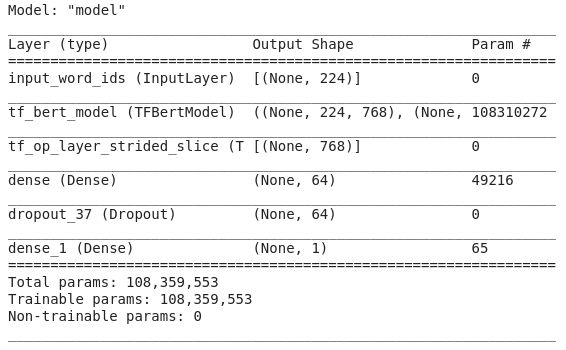
We pass the Dataset object into the model and start training.

n_steps = x_train.shape[0] // BATCH_SIZE
train_history = model.fit(
    train_dataset,
    steps_per_epoch=n_steps,
    validation_data=valid_dataset,
    epochs=EPOCHS
)

Now that the model is trained. We can visualize the training history using the following function.

from matplotlib import pyplot as plt
def plot_loss(his, epoch, title):
    plt.style.use('ggplot')
    plt.figure()
    plt.plot(np.arange(0, epoch), his.history['loss'], label='train_loss')

    plt.plot(np.arange(0, epoch), his.history['val_loss'], label='val_loss')

    plt.title(title)
    plt.xlabel('Epoch #')
    plt.ylabel('Loss')
    plt.legend(loc='upper right')
    plt.show()

plot_loss(train_history, EPOCHS, "training loss")

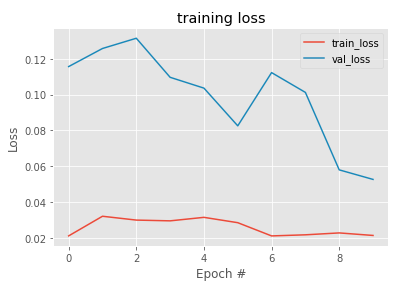
The training history shows that although there is a bump from Epoch 5 to Epoch 6 for the validation loss, the overall loss for both train and validation decreases gradually.

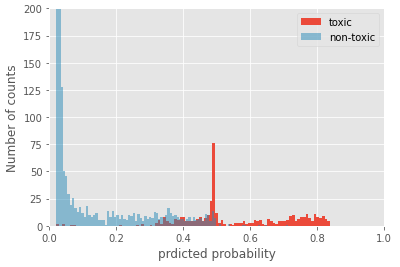
Also, we can look at the distributions of the prediction probabilities on the validation set. It indicates that if the predicted probability is below 0.3, the comment is more likely to be non-toxic. In contrast, a probability of above 0.6 will predict toxic for the comment. In the probability region between those two, there is some overlap, which means it is challenging to predict the nature of the comment if it falls into this intermediate region.

Model Refinement

Next we will discussion various techniques to improve the model performance.

Model Architectures

The model architecture is mainly associated with the “Multilingual Issue”. Since different architectures are pre-trained on varying size dataset and targeted on different semi-unsupervised tasks, their capability of mining cross-lingual knowledge is different.

The Basic BERT model performs not too bad on this multilingual task, which has a public LB score of around 0.916. As we mentioned in the second blog, the most successful multilingual model is probably the XLM-RoBERTa model, especially the large XLM-R model. The large XLM-R model has more than 500 million parameters, and it demonstrates to be superior to other language models in multilingual modeling. With XLM-R architecture, our baseline LB score goes up to 0.9365, a significant improvement compared to BERT.

Hyperparameter Tuning

The hyperparameter tuning aims to the resolve the “Data Size Issue” and “Unbalance Issue”. However, we are not able to tune too many hyperparameters due to such a limited time for this final project. Instead, I will elaborate the techniques I tried and the reasoning.

• Adjust the maximum length for the input vector sequence. I tried lengths of 150, 192, 210, and 224. 224 maximum length gives the best LB score of 0.9378.

• Change the data size of training set. Only a fraction of the training data corresponding to non-toxic comments is selected. It was found that sub-sampling the non-toxic comments help a lot in balancing the dataset. It increases the LB score to 0.9401 with the best maximum length.

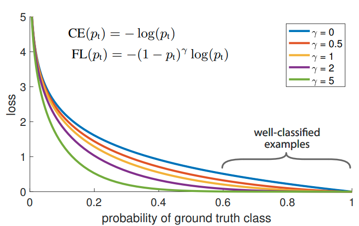
• Tweak the loss function. The most typical loss function for a binary classification problem is the binary_crossentropy as implemented in Tensorflow. Yet, a great work by Lin et.al proves that a novel loss they term “Focal Loss” that adds a pre-factor to the standard cross entropy criterion can boost the model accuracy. The name “focal” comes from the fact that the model now pays less attention to the well classified samples while putting more focus on hard, misclassified examples. A weighting factor is also introduced to mitigate the class unbalance issue. The figure below shows why Focal loss focuses more on the misclassified data. Unfortunately, models with focal loss perform similarly compared to the standard binary cross entropy.

• Other random efforts. We add an additional dense layer and a dropout layer right ahead of the final layer. Then the dropout rate and the number of nodes in the dense layer are tuned. Although the model does not improve a lot in terms of the validation accuracy and the LB score, we believe that it will be helpful because adding regularization into a model will increase the generalization capability on unseen data. Moreover, I also tried a learning rate scheduler. However, no significant improvement was observed.

Data Augmentation

This strategy is of central importance as in the training data we only have English-written comments while in the validation and test set, we have comments written in other languages. Although the multilingual model can capture some of the shared knowledge between various languages, data augmentation is necessary to improve the model performance. As of now, two approaches are tested.

• Translate the training set to other languages and keep the validation and test set unchanged. This approach gives me a best LB score of 0.9365.

• Translate the validation and test set to English. This model performs a little better, with a LB score of 0.9378.

Ensemble Magic

I did weighted ensemble on four models. The LB score for individual models are 0.9427, 0.9416, 0.9401 and 0.9365, respectively. By carefully tuning the weights, I arrived at a LB score of 0.9453.

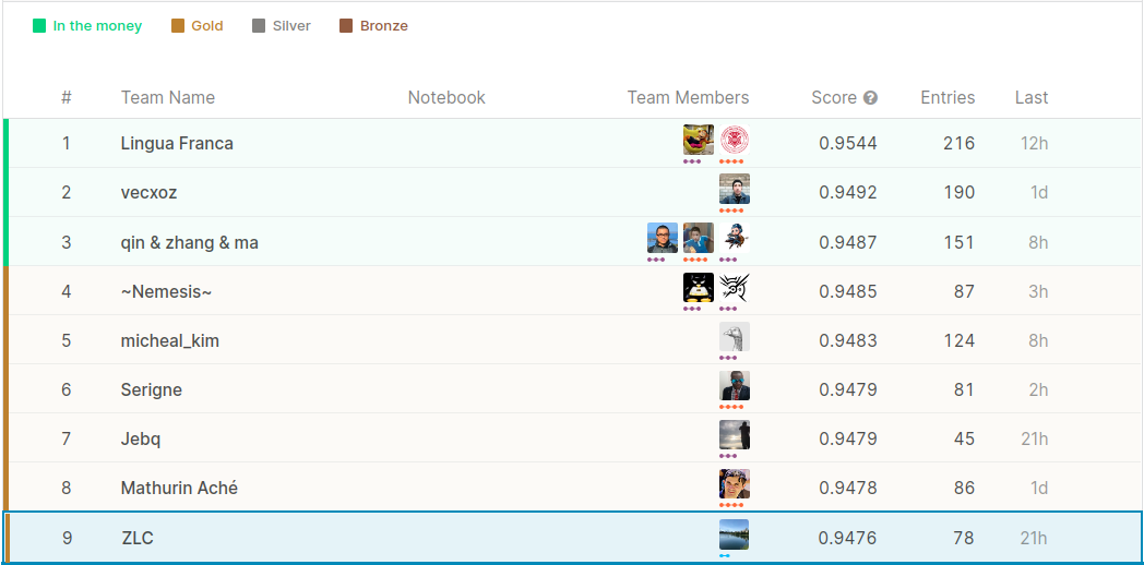
Further combining my own best submission with public top-score submissions, I am able to achieve a Public LB score of 0.9476, which leads to a top 5% position out of more than 800 teams. The following snapshot for the Public ranking is taken on May 6th.

Next steps

• Metric learning: post process the prediction to further improve the ranking on public leaderboard.

• Transfer learning: using the trained model for other purposes such as predicting the state of a reddit post, which can be mainly categorized as upvote and downvote.

Annotated Citations

• Jay Alammer. (2019, November 26). A Visual Guide to Using BERT for the First Time. Retrieved from BERT notebook. The vivid figures for illustration of key components in a language model are taken from this awesome blog.

• Jacob Devlin, Ming-Wei Chang, Kenton Lee and Kristina Toutanova. BERT: Pre-training of Deep Bidirectional Transformers for Language Understanding. 2019. This is the original paper for the basic BERT model.

• Tsung-Yi Lin et al. Focal Loss for Dense Object Detection. 2017. This paper introduces the idea of using Focal Loss to make the model focus more on those misclassified images.